Reading and writing data

A short description of the post.

1. load the packages we will use

library(tidyverse)
library(here)
library(janitor)
library(skimr)

2. Download \(CO_2\) emissions per capita from Our world in Data into the directory for this post.

3. Assign the location of the file to filve_csv. The data should be in the same directory as this file

Read the data into R and assign it to emissions

file_csv  <- here("_posts",
                 "2022-02-21-reading-and-writing-data",
                 "co-emissions-per-capita.csv")

emissions  <- read_csv(file_csv)

2. Show the first 10 rows (observations of) emissions

emissions

# A tibble: 23,307 × 4
   Entity      Code   Year `Annual CO2 emissions (per capita)`
   <chr>       <chr> <dbl>                               <dbl>
 1 Afghanistan AFG    1949                              0.0019
 2 Afghanistan AFG    1950                              0.0109
 3 Afghanistan AFG    1951                              0.0117
 4 Afghanistan AFG    1952                              0.0115
 5 Afghanistan AFG    1953                              0.0132
 6 Afghanistan AFG    1954                              0.013 
 7 Afghanistan AFG    1955                              0.0186
 8 Afghanistan AFG    1956                              0.0218
 9 Afghanistan AFG    1957                              0.0343
10 Afghanistan AFG    1958                              0.038 
# … with 23,297 more rows

5. Start with emissions

• use clean_names from the janitor package to make the names easier to work with
• assign the output to tidy_emissions
• show the first 10 rows of tidy_emissions

tidy_emissions   <- emissions %>%
  clean_names()

tidy_emissions

# A tibble: 23,307 × 4
   entity      code   year annual_co2_emissions_per_capita
   <chr>       <chr> <dbl>                           <dbl>
 1 Afghanistan AFG    1949                          0.0019
 2 Afghanistan AFG    1950                          0.0109
 3 Afghanistan AFG    1951                          0.0117
 4 Afghanistan AFG    1952                          0.0115
 5 Afghanistan AFG    1953                          0.0132
 6 Afghanistan AFG    1954                          0.013 
 7 Afghanistan AFG    1955                          0.0186
 8 Afghanistan AFG    1956                          0.0218
 9 Afghanistan AFG    1957                          0.0343
10 Afghanistan AFG    1958                          0.038 
# … with 23,297 more rows

6. Start with the tidy_emissions THEN

• use filter to extract rows with year == 2018 THEN
• use skim to calculate the descriptive statistics

tidy_emissions  %>%
  filter(year == 2018)  %>%
  skim

Table 1: Data summary

Name	Piped data
Number of rows	229
Number of columns	4
_______________________
Column type frequency:
character	2
numeric	2
________________________
Group variables	None

Variable type: character

skim_variable	n_missing	complete_rate	min	max	empty	n_unique	whitespace
entity	0	1.00	4	32	0	229	0
code	12	0.95	3	8	0	217	0

Variable type: numeric

skim_variable	n_missing	complete_rate	mean	sd	p0	p25	p50	p75	p100	hist
year	0	1	2018.00	0.00	2018.00	2018.00	2018.0	2018.00	2018.00	▁▁▇▁▁
annual_co2_emissions_per_capita	0	1	5.03	5.63	0.03	0.99	3.5	6.85	38.44	▇▂▁▁▁

7. 13 observations have a missing code. How are these observations different? start with tidy_emissions then extract rows with year == 2018 and are missing a code

tidy_emissions  %>%
  filter(year == 2018, is.na(code))

# A tibble: 12 × 4
   entity                     code   year annual_co2_emissions_per_ca…
   <chr>                      <chr> <dbl>                        <dbl>
 1 Africa                     <NA>   2018                         1.09
 2 Asia                       <NA>   2018                         4.44
 3 Asia (excl. China & India) <NA>   2018                         4.14
 4 EU-27                      <NA>   2018                         6.85
 5 EU-28                      <NA>   2018                         6.70
 6 Europe                     <NA>   2018                         7.48
 7 Europe (excl. EU-27)       <NA>   2018                         8.39
 8 Europe (excl. EU-28)       <NA>   2018                         9.15
 9 North America              <NA>   2018                        11.4 
10 North America (excl. USA)  <NA>   2018                         4.80
11 Oceania                    <NA>   2018                        11.4 
12 South America              <NA>   2018                         2.58

Entities that are not countries do not have country codes

8. Start with tidy_emissions THEN

   use filter to extract rows with year == 2018 and without missing codes THEN use select to drop the year variable THEN use rename to chnage the variable entity to country assign the output to emissions_2018

emissions_2018  <- tidy_emissions  %>%
  filter(year == 2018, !is.na(code))   %>%
  select(-year)  %>%
  rename(country = entity)

9. Which 15 countries have the highest per_capita_co2_emissions?

start with emissions_2018 THEN use slice_max to extract the 15 rows with the per_capita_co2_emissions assign the output to max_15_emitters

max_15_emitters  <- emissions_2018  %>%
  slice_max(annual_co2_emissions_per_capita, n = 15)

10. Which 15 countries have the lowest per_capita_co2_emissions?

start with emissions_2018 THEN use slice_min to extract the 15 rows with the lowest values assign the output to min_15_emitters

min_15_emitters  <- emissions_2018  %>%
  slice_min(annual_co2_emissions_per_capita, n = 15)

11. Use bind_rows to bind together the max_15_emitters and min_15_emitters assign the output to max_min_15

max_min_15  <- bind_rows(max_15_emitters, min_15_emitters)

12. Export `max_min_15 to 3 files formats

max_min_15  %>% write_csv("max_min_15.csv") # comma-separates values
max_min_15  %>% write_tsv("max_min_15.tsv")  # tab separated
max_min_15  %>% write_delim("max_min_15.psv", delim ="|") #pipe-separated

13. Read the file 3 file formats into R

max_min_15_csv <-   read_csv("max_min_15.csv") # comma-separated values
max_min_15_tsv <-   read_tsv("max_min_15.tsv")  # tab separated
max_min_15_psv <-   read_delim("max_min_15.psv", delim = "|") #piper-separated

14. Use setdiff to check for any differences among max_min_15_csv, max_min_15_tsv and max_min_15_psv

setdiff(max_min_15_csv, max_min_15_tsv)

# A tibble: 0 × 3
# … with 3 variables: country <chr>, code <chr>,
#   annual_co2_emissions_per_capita <dbl>

Are there any differences?

15. Reorder country in max_min_15 for plotting and assign to max_min_15_plot_data

start with emissions_2019 THEN use mutate to reorder country according to per_capital_co2_emissions

max_min_15_plot_data  <- max_min_15 %>%
  mutate(country = reorder(country, annual_co2_emissions_per_capita))

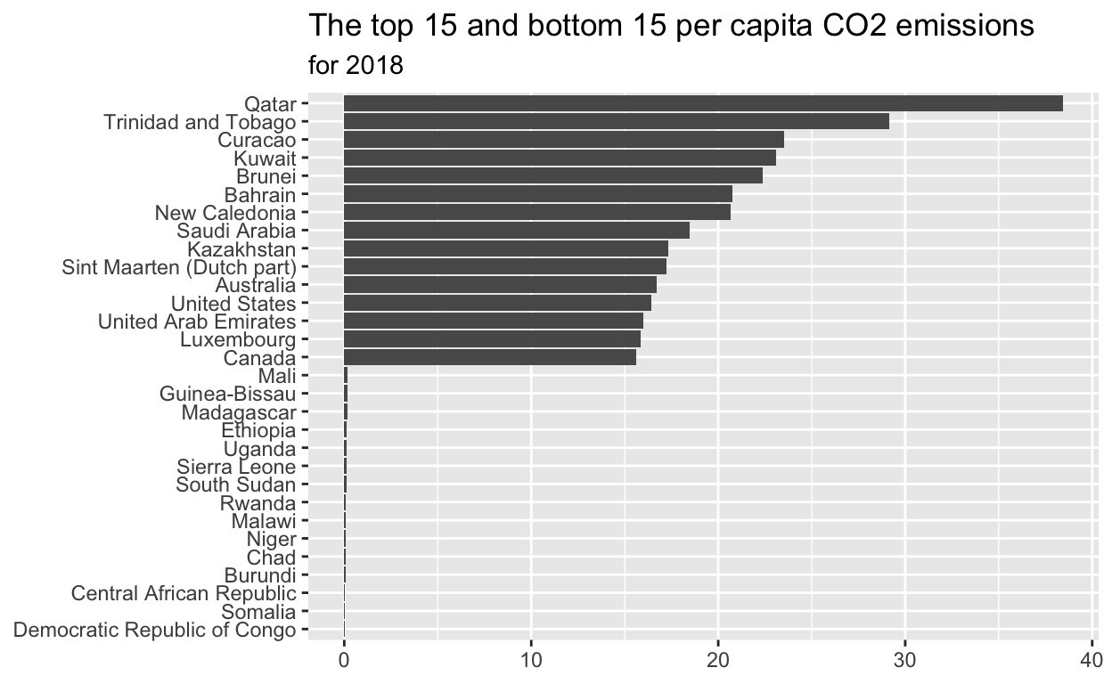
16. Plot max_min_15_plot_data

ggplot(data = max_min_15_plot_data,
       mapping = aes(x = annual_co2_emissions_per_capita,y = country)) +
  geom_col() +
  labs(title = "The top 15 and bottom 15 per capita CO2 emissions",
       subtitle = "for 2018",
       x = NULL,
       y = NULL)

17. Save the plot directory with this post

ggsave(filename = "preview.png", 
       path = here("_posts", "2022-02-21-reading-and-writing-data"))

18. Add preview.png to yaml chuck at the top of this file

preview: preview.png